Lecture notes — Basics of a Turing Machine
ver. 1.1.1
Where we are
This is the first unit of the module, so nothing is assumed from an earlier one. What we do assume is comfort with a little discrete mathematics: sets, tuples, functions, and reading a table that says “in this situation, do that”.
This course does not have formal language theory as a prerequisite, and this unit is written to need none. We will not use finite automata, pushdown automata, grammars, or the classification of languages as regular or context-free. Everything is built from scratch: we define the machine, and every claim about what it can do is backed by building one.
We are after one thing: a precise answer to what is a computation? You already know how to program, which means you have a working intuition for it. An intuition is not enough. The next unit proves that certain problems have no algorithm at all, and you cannot prove the absence of something you have not defined.
What you will be able to do
explain-turing-model-of-computation— Explain how a Turing machine formalizes a human computing with pencil and paper.state-the-formal-definition— Write down the 6-tuple definition of a Turing machine and read a transition function.trace-a-computation-as-configurations— Trace a Turing machine’s run as a sequence of configurations under the yield relation.construct-a-transforming-machine— Construct a Turing machine that rewrites its tape, such as erasing or copying a string.construct-a-recognizer— Construct a Turing machine that accepts a given language, including one whose strings must be counted three ways at once.explain-the-universal-turing-machine— Explain what a Universal Turing Machine does and why encoding a machine as data is what makes it possible.
What we will cover
- Turing Machine — a formal model of computation: an infinite tape, a read/write head, and a finite state control.
- Turing Machine Configuration — a snapshot of the state, the head position and the tape contents at one step.
- Universal Turing Machine — a machine that simulates the execution of any other machine on any input.
- Compiler Self-Hosting and Bootstrapping — writing a language’s compiler in the very language it compiles.
Why we need a model of computation
We start with the question the whole module answers: what does it mean for something to be computable?
You can already write programs, and you have a sense of which tasks a program can do. That sense will not survive contact with the next unit, which proves that some problems have no program at all. Before we can prove a problem cannot be solved, we need a definition of “solved” precise enough to argue about.
The definition has to satisfy three demands at once, and they pull against each other:
- simple enough to reason about mathematically — if the model has fifty features, no proof about it will ever finish;
- intuitive enough that we believe it captures what a person does when computing by hand;
- generic enough that nothing computable escapes it.
Turing’s answer was to model the person, not the machine. Rather than inventing a powerful device and hoping it was powerful enough, he looked at what a human being actually does with a pencil and a sheet of paper, and formalized that.
In this unit we will derive that model, define it precisely, trace it running, build four of them, and finish with the Universal Turing Machine — a machine that runs other machines.
We do not yet ask what Turing machines cannot do. That is the next unit’s subject. Here we build the object it will reason about.
Learning outcomes
- explain-turing-model-of-computation: Explain how a Turing machine formalizes a human computing with pencil and paper.
From paper to tape
Turing set himself the aim of designing a model that is simple, intuitive, generic, and formalizes the computation performed by a human mind. So let’s start where he did, with a person doing arithmetic on paper. What do they actually do?
- write the input on the paper;
- do the computation — think, and write intermediate results on the paper;
- write the output on the paper.
Now we map each piece onto a machine component. A Turing machine is the result: an infinite tape, a read/write head, and a finite state control.
| Human computation | Machine computation |
|---|---|
| the paper | tape |
| the hand and eye | tape head |
| what to do next | transition function |
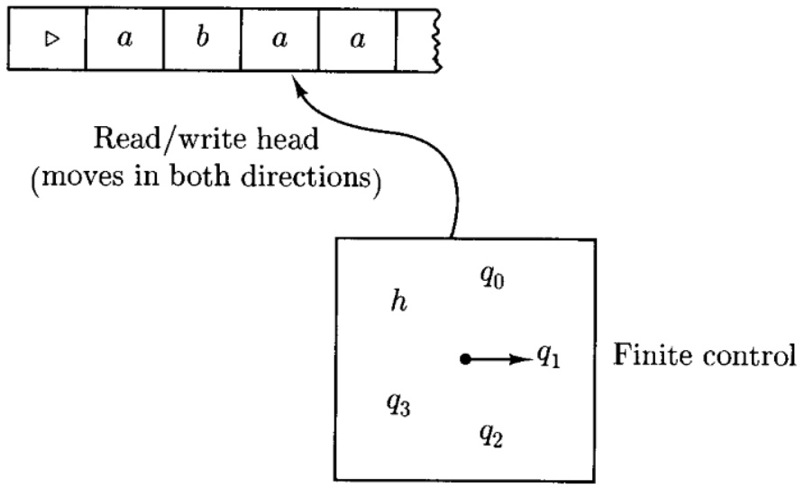
Each part earns its place:
Tape — simulates unlimited sheets of paper for computation.
Unlimited, not infinite in use. Any run that halts has touched finitely many cells; the tape just never runs out.
Tape head — reads and writes onto a tape cell, and moves left or right.
One cell at a time, which is exactly the constraint a person writing by hand is under.
States — simulate the states of a human mind.
There are finitely many. This is the substantive assumption in the whole model, and it is what makes the model analysable.
Input — a finite number of symbols initially on the tape. Output — a finite number of symbols finally on the tape.
Computation — state transitions based on rules and input symbols.
From this, exactly three primitive operations follow:
| Operation | Explanation |
|---|---|
| Write | (Optionally) writes a new symbol at the current tape position. |
| Move | (Optionally) moves either left or right. |
| Think | (Optionally) changes to a new state. |
Everything in the rest of this unit is built from those three.
The tape-and-head diagrams here follow Lewis and Papadimitriou, Elements of the Theory of Computation, which is the source the slides cite for them.
The claim that write, move and think capture every mechanical computation is not a theorem. It is a claim about the physical world, and it cannot be proved. We will meet it by name in the next unit as the Church–Turing thesis.
Learning outcomes
- explain-turing-model-of-computation: Explain how a Turing machine formalizes a human computing with pencil and paper.
Concepts
- turing-machine: derived here from human pencil-and-paper computation, giving the tape, the head and the finite state control
The formal definition
Now we turn the analogy into a definition.
A Turing machine \(M\) is a 6-tuple
\[M = (Q, \Sigma, \Gamma, \delta, q_0, H)\]
where:
- \(Q\) — a finite set, the set of states.
- \(\Sigma\) — a finite set, the input alphabet. \(\Sigma\) excludes \(\triangleright, \square, \leftarrow, \rightarrow\).
- \(\Gamma\) — a finite set, the tape alphabet, with \(\Sigma \cup \{\triangleright, \square\} \subseteq \Gamma\). \(\Gamma\) excludes \(\leftarrow, \rightarrow\).
- \(\delta : (Q - H) \times \Gamma \to Q \times (\Gamma \cup \{\leftarrow, \rightarrow\})\) — the transition function, such that the tape head never falls off the tape and never erases the \(\triangleright\) symbol.
- \(q_0\) — the start state, \(q_0 \in Q\).
- \(H = \{q_{\text{acc}}, q_{\text{rej}}\}\) — the set of halting states, \(H \subseteq Q\).
The symbols
- \(\triangleright\) — the left end symbol.
- \(\square\) — the blank symbol.
- \(\leftarrow, \rightarrow\) — the left and right movement symbols.
- \(\Sigma\) — input, output and special symbols.
- \(\Gamma\) — every symbol that can appear on the tape.
The reason \(\Gamma\) is allowed to be bigger than \(\Sigma\) matters more than it looks. The extra symbols are working space: marks the machine writes to remember what it has already dealt with. Every machine we build below uses them.
Reading the transition function
Two details in \(\delta\) are worth slowing down for.
- Its domain is \((Q - H) \times \Gamma\), not \(Q \times \Gamma\). Halting states have no outgoing transitions. That is precisely what “halting” means: \(M\) stops when it reaches an accept or a reject state, because \(\delta\) is not defined there.
- Its codomain is \(Q \times (\Gamma \cup \{\leftarrow, \rightarrow\})\). A single step produces a next state paired with either a symbol to write or a direction to move — never both. Writing and moving take two steps.
There is one more constraint, and it is a condition on \(\delta\) rather than part of its type: \(M\) never falls off the left end of the tape. When the current symbol is \(\triangleright\), the head has to move right.
Forgetting the \(\triangleright\) column. Every machine in this unit begins with a transition on \(\triangleright\) that moves right, and a machine that omits it is not a legal Turing machine at all.
We will read every machine below in two notations — a transition table and a state diagram — and you should be able to move between them.
Learning outcomes
- state-the-formal-definition: Write down the 6-tuple definition of a Turing machine and read a transition function.
Concepts
- turing-machine: pinned down here as the 6-tuple \(M = (Q, \Sigma, \Gamma, \delta, q_0, H)\), with the constraints that make \(\delta\) well formed
Configurations and the yield relation
We have defined the machine. Now we need a way to talk about a run of it.
A Turing Machine Configuration is the information about the current state, the tape head position, and the tape content — for example \((q_4, \triangleright bbb\square)\). It is a snapshot: everything you would need to pause the machine and resume it later, and nothing more.
A computation is a sequence of successive configurations. Here is a complete run, of a machine we will build in a moment, on the input \(bbb\):
| Time | Configuration | State | Tape |
|---|---|---|---|
| 0 | \(C_0\) | \(q_0\) | ▷ b b b □ □ … |
| 1 | \(C_1\) | \(q_1\) | ▷ b b b □ □ … |
| 2 | \(C_2\) | \(q_4\) | ▷ b b b □ □ … |
| 3 | \(C_3\) | \(q_4\) | ▷ b b b □ □ … |
| 4 | \(C_4\) | \(q_4\) | ▷ b b b □ □ … |
| 5 | \(C_5\) | \(q_{\text{rej}}\) | ▷ b b b □ □ … |
We write one configuration yielding the next with \(\vdash_M\):
\[C_0 \vdash_M C_1 \vdash_M C_2 \vdash_M C_3 \vdash_M C_4 \vdash_M C_5\]
The notation compresses in two ways. The computation time — its length — is 5 here, written
\[C_0 \vdash^{5}_{M} C_5\]
and when the number of steps does not matter, \(C_1 \vdash^{*}_{M} C_4\) says only that the first yields the second eventually.
Configurations get names according to where they sit in a run: the starting configuration, and the accepting, rejecting and halting configurations.
Tracing by hand, one configuration per line, is slow. It is meant to be. It is the only way to see what a machine actually does rather than what you meant it to do, and it is how you will debug every machine you build in the next two sections.
A Turing machine may reach \(q_{\text{acc}}\) before the head has visited the whole input, so it can accept a string it has not entirely read. Nothing obliges the head to advance through the input at a fixed rate, or at all — it moves only where \(\delta\) sends it. That freedom is what makes both early acceptance and running forever possible.
Learning outcomes
- trace-a-computation-as-configurations: Trace a Turing machine’s run as a sequence of configurations under the yield relation.
Concepts
- configuration: used here to define a run, as the chain of snapshots related by \(\vdash_M\)
Machines that rewrite the tape
Our first two machines do not answer questions. They compute: they change the tape and leave a result on it. This is the cleanest way to see what the rewritable tape buys us, because a machine that could only ever read would have nowhere to put an answer.
Erasing the input
Problem. Construct a TM to erase the input string.
The machine sweeps right, replacing each symbol with a blank. Here is the run on \(aaa\):
| Time | State | Tape |
|---|---|---|
| 0 | \(q_0\) | ▷ a a a □ … |
| 1 | \(q_0\) | ▷ a a a □ … |
| 2 | \(q_1\) | ▷ □ a a □ … |
| 3 | \(q_0\) | ▷ □ a a □ … |
| 4 | \(q_1\) | ▷ □ □ a □ … |
| 5 | \(q_0\) | ▷ □ □ a □ … |
| 6 | \(q_1\) | ▷ □ □ □ □ … |
| 7 | \(q_0\) | ▷ □ □ □ □ … |
| 8 | \(q_h\) | ▷ □ □ □ □ … |
Two states are enough, because the work alternates: \(q_0\) writes a blank over the current symbol, \(q_1\) steps right, and back again.
| \(\triangleright\) | \(a\) | \(\square\) | |
|---|---|---|---|
| \(q_0\) | \((q_0, \rightarrow)\) | \((q_1, \square)\) | \((q_h, \square)\) |
| \(q_1\) | — | \((q_0, a)\) | \((q_0, \rightarrow)\) |
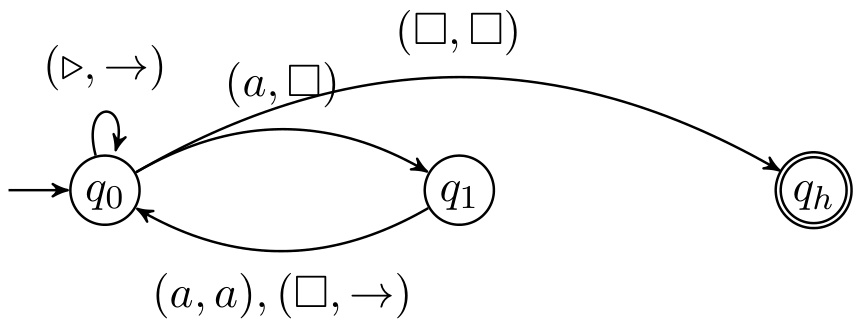
Read the first row against the definition. On \(\triangleright\) the machine moves right — the constraint from the previous section, in force. On \(a\) it writes \(\square\). On \(\square\) it writes \(\square\) and halts, because there is nothing left to erase.
Copying a string
Problem. Construct a Turing machine that copies a string from the language \(L = \Sigma^*\) where \(\Sigma = \{a, b\}\).
This one is harder, and it introduces the technique we reuse for the rest of the unit. The tape alphabet grows to give the machine somewhere to keep its place:
\[\Gamma = \Sigma \cup \{\triangleright, \square, \#, 1, 2\}\]
\(\#\) marks where the copy begins. The symbols \(1\) and \(2\) are markers: \(1\) stands for an \(a\) already copied, \(2\) for a \(b\) already copied. The strategy is one symbol per round trip — mark it, walk right to the end, write the copy, walk back, restore the marker, step right.
| \(\triangleright\) | \(a\) | \(b\) | \(\#\) | 1 | 2 | \(\square\) | |
|---|---|---|---|---|---|---|---|
| \(q_0\) | \((q_1, \rightarrow)\) | — | — | — | — | — | — |
| \(q_1\) | — | \((q_1, \rightarrow)\) | \((q_1, \rightarrow)\) | — | — | — | \((q_2, \#)\) |
| \(q_2\) | \((q_3, \rightarrow)\) | \((q_2, \leftarrow)\) | \((q_2, \leftarrow)\) | \((q_2, \leftarrow)\) | — | — | — |
| \(q_3\) | — | \((q_4, 1)\) | \((q_5, 2)\) | \((q_{\text{acc}}, \#)\) | — | — | — |
| \(q_4\) | — | \((q_4, \rightarrow)\) | \((q_4, \rightarrow)\) | \((q_4, \rightarrow)\) | \((q_4, \rightarrow)\) | — | \((q_6, a)\) |
| \(q_5\) | — | \((q_5, \rightarrow)\) | \((q_5, \rightarrow)\) | \((q_5, \rightarrow)\) | — | \((q_5, \rightarrow)\) | \((q_6, b)\) |
| \(q_6\) | — | \((q_6, \leftarrow)\) | \((q_6, \leftarrow)\) | \((q_6, \leftarrow)\) | \((q_7, a)\) | \((q_7, b)\) | — |
| \(q_7\) | — | \((q_3, \rightarrow)\) | \((q_3, \rightarrow)\) | — | — | — | — |
Cells with “—” mean the TM terminates in \(q_{\text{rej}}\).
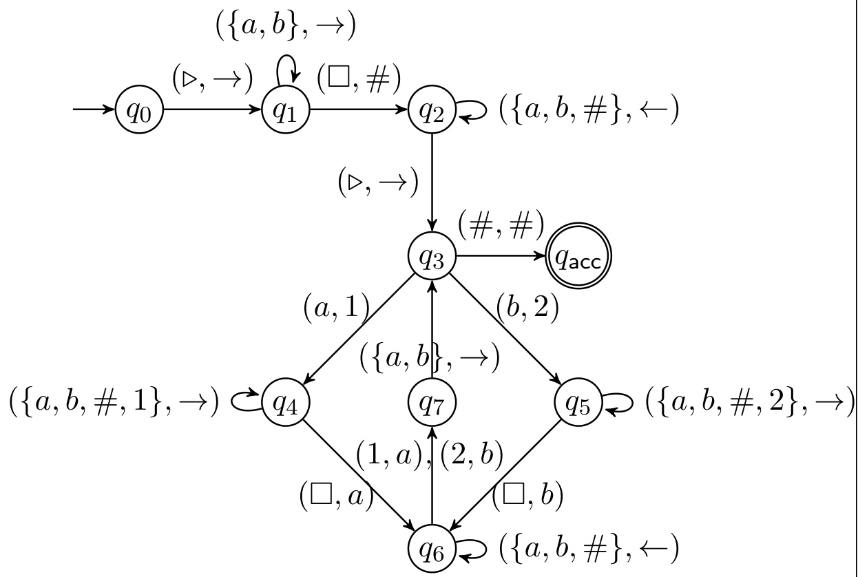
Two ideas generalise from this, and both come back in the next section:
Markers are memory. The state set is finite and cannot count, so anything the machine must remember about position gets written on the tape instead.
That is what \(1\) and \(2\) are for. They also record which symbol was there, so \(q_7\) can restore it.
A round trip is a pair of states. \(q_4\) and \(q_5\) go right; \(q_6\) comes back.
Every multi-pass machine has this shape. Recognising it is most of reading one.
Learning outcomes
- construct-a-transforming-machine: Construct a Turing machine that rewrites its tape, such as erasing or copying a string.
- trace-a-computation-as-configurations: Trace a Turing machine’s run as a sequence of configurations under the yield relation.
Machines that recognize languages
Now we build machines that answer questions. The two examples sit either side of an interesting line: what a single scan can settle, and what it cannot.
One scan is enough
Problem. Construct a Turing machine that accepts all strings from the language \(L = \{\text{strings containing } ab \text{ or ending with } ba\}\).
| \(\triangleright\) | \(a\) | \(b\) | \(\square\) | |
|---|---|---|---|---|
| \(q_0\) | \((q_1, \rightarrow)\) | — | — | — |
| \(q_1\) | — | \((q_2, \rightarrow)\) | \((q_4, \rightarrow)\) | — |
| \(q_2\) | — | \((q_2, \rightarrow)\) | \((q_3, \rightarrow)\) | — |
| \(q_3\) | — | \((q_{\text{acc}}, \rightarrow)\) | \((q_{\text{acc}}, \rightarrow)\) | \((q_{\text{acc}}, \rightarrow)\) |
| \(q_4\) | — | \((q_5, \rightarrow)\) | \((q_4, \rightarrow)\) | — |
| \(q_5\) | — | \((q_2, \rightarrow)\) | \((q_3, \rightarrow)\) | \((q_{\text{acc}}, \rightarrow)\) |
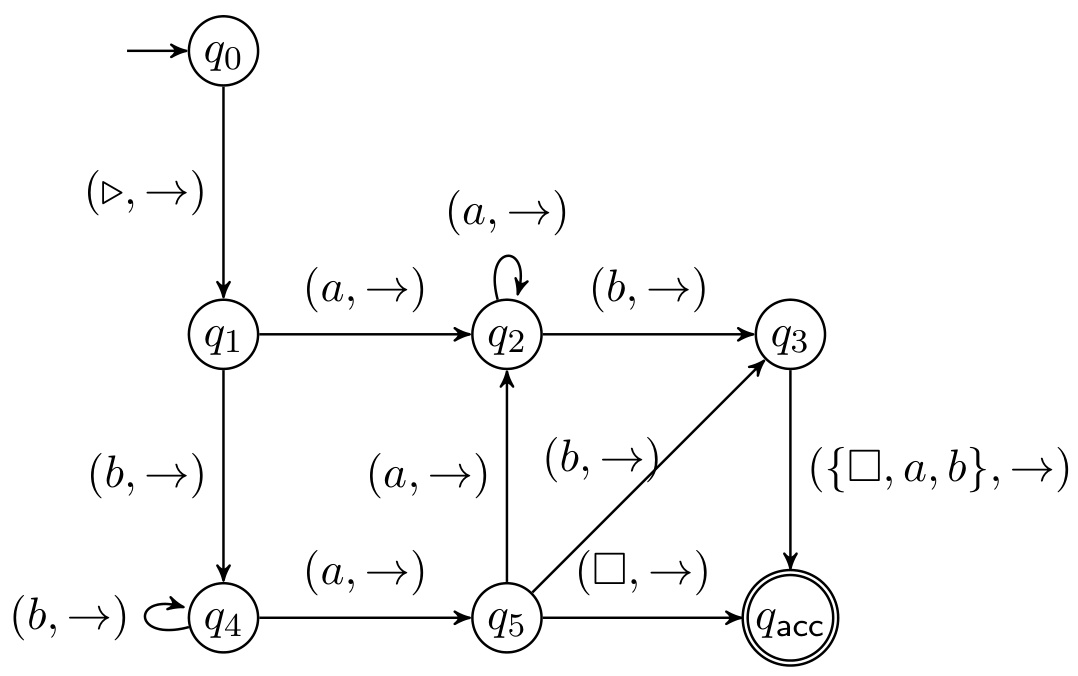
Notice what the table does not contain: there is no write anywhere in it. Every entry is a move. The whole job is done by the finite state set — \(q_2\) means “just saw an \(a\)”, \(q_4\) means “just saw a \(b\)”, \(q_3\) means “have seen \(ab\), accept whatever follows”.
The run on \(bba\), which is accepted:
| Time | State | Tape |
|---|---|---|
| 0 | \(q_0\) | ▷ b b a □ □ … |
| 1 | \(q_1\) | ▷ b b a □ □ … |
| 2 | \(q_4\) | ▷ b b a □ □ … |
| 3 | \(q_4\) | ▷ b b a □ □ … |
| 4 | \(q_5\) | ▷ b b a □ □ … |
| 5 | \(q_{\text{acc}}\) | ▷ b b a □ □ … |
And on \(bbb\), which is rejected — this is the run we traced as configurations earlier:
| Time | State | Tape |
|---|---|---|
| 0 | \(q_0\) | ▷ b b b □ □ … |
| 1 | \(q_1\) | ▷ b b b □ □ … |
| 2 | \(q_4\) | ▷ b b b □ □ … |
| 3 | \(q_4\) | ▷ b b b □ □ … |
| 4 | \(q_4\) | ▷ b b b □ □ … |
| 5 | \(q_{\text{rej}}\) | ▷ b b b □ □ … |
Now trace \(aabbbbb\) yourself. The machine reaches \(q_3\) after reading \(aab\) and accepts on the next step — with four symbols still unread. A Turing machine can accept a string without scanning it completely.
Use the machine to check acceptance of \(\epsilon\), \(aba\), \(aaa\), \(aab\) and \(baa\). Which of them reach \(q_{\text{acc}}\), and after how many steps?
When one scan is not enough
Problem. Construct a Turing machine to accept all strings from the language \(L = \{a^n b^n c^n \mid n \geq 1\}\), so \(L = \{abc, aabbcc, aaabbbccc, \ldots\}\).
Here the state set alone will not do, and it is worth seeing exactly why. The machine must confirm that three counts are equal; \(n\) can be arbitrarily large; and \(Q\) is finite. No fixed number of states can hold an unbounded tally. The counting has to happen on the tape.
So we grow the alphabet again:
\[\Gamma = \Sigma \cup \{\triangleright, \square, x, y, z\}\]
with \(x\), \(y\) and \(z\) marking a crossed-off \(a\), \(b\) and \(c\). Each pass crosses off one of each and returns to the left end:
| \(\triangleright\) | \(a\) | \(b\) | \(c\) | \(x\) | \(y\) | \(z\) | \(\square\) | |
|---|---|---|---|---|---|---|---|---|
| \(q_0\) | \((q_1, \rightarrow)\) | — | — | — | — | — | — | — |
| \(q_1\) | — | \((q_2, x)\) | — | — | — | \((q_5, \rightarrow)\) | — | — |
| \(q_2\) | — | \((q_2, \rightarrow)\) | \((q_3, y)\) | — | \((q_2, \rightarrow)\) | \((q_2, \rightarrow)\) | — | — |
| \(q_3\) | — | — | \((q_3, \rightarrow)\) | \((q_4, z)\) | — | \((q_3, \rightarrow)\) | \((q_3, \rightarrow)\) | — |
| \(q_4\) | — | \((q_4, \leftarrow)\) | \((q_4, \leftarrow)\) | — | \((q_1, \rightarrow)\) | \((q_4, \leftarrow)\) | \((q_4, \leftarrow)\) | — |
| \(q_5\) | — | — | — | — | — | \((q_5, \rightarrow)\) | \((q_5, \rightarrow)\) | \((q_{\text{acc}}, \square)\) |
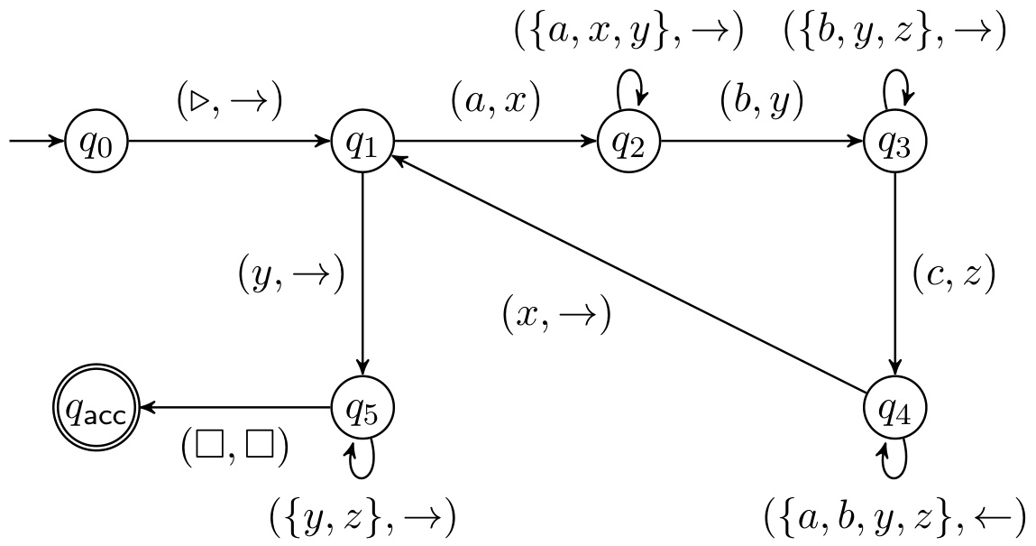
Follow the cycle: \(q_1\) crosses an \(a\) to \(x\), \(q_2\) runs right to the first \(b\) and crosses it to \(y\), \(q_3\) runs right to the first \(c\) and crosses it to \(z\), and \(q_4\) walks all the way back to the last \(x\) and hands over to \(q_1\) for the next pass. When \(q_1\) finds \(y\) instead of \(a\) the \(a\)s have run out, and \(q_5\) sweeps right to confirm only \(y\)s and \(z\)s remain before accepting.
Here is \(aabbcc\), one row per pass boundary:
| State | Tape |
|---|---|
| \(q_0\) | ▷ a a b b c c □ |
| \(q_2\) | ▷ x a b b c c □ |
| \(q_3\) | ▷ x a y b c c □ |
| \(q_4\) | ▷ x a y b z c □ |
| \(q_2\) | ▷ x x y b z c □ |
| \(q_3\) | ▷ x x y y z c □ |
| \(q_4\) | ▷ x x y y z z □ |
| \(q_5\) | ▷ x x y y z z □ |
| \(q_{\text{acc}}\) | ▷ x x y y z z □ |
The crossings-off are the memory. They persist between passes, so pass \(k\) can see what pass \(k-1\) did, and a machine with six states matches three counts of any size. It is the same trick as the copying machine, applied to a harder problem.
Key ideas
- A recognizer needs no writes when the finite state set can hold everything it must remember.
- When it cannot — an unbounded count — the tape holds the memory instead, as crossed-off symbols.
- Rejection is a state, \(q_{\text{rej}}\), reached by every transition the table leaves blank.
Check acceptance of \(abc\), \(aa\), \(c\), \(abbc\), \(aabc\), \(abcc\) and \(\epsilon\). Then construct a machine for \(L = \{a^n b^n c^n \mid n \geq 0\}\) — the change is smaller than it looks, but it is not nothing.
Learning outcomes
- construct-a-recognizer: Construct a Turing machine that accepts a given language, including one whose strings must be counted three ways at once.
- trace-a-computation-as-configurations: Trace a Turing machine’s run as a sequence of configurations under the yield relation.
The Universal Turing Machine
Every machine so far has done exactly one job. The last construction of the unit does all of them.
A Universal Turing Machine \(U\) can simulate the execution of any Turing machine \(M\) on any input \(w\). We write the input to \(U\) as \(\langle M, w \rangle\) — an encoding of the machine, together with that machine’s input.
Its specification is a list of promises:
- \(U(\langle M, w \rangle)\) halts if and only if \(M\) halts on input \(w\).
- If \(M\) is a deciding or semideciding machine, then if \(M\) accepts, \(U\) accepts; if \(M\) rejects, \(U\) rejects.
- If \(M\) computes a function, then \(U(\langle M, w \rangle)\) must equal \(M(w)\).
And the theorem that says this is achievable:
Given any Turing machine \(M\) and an input string \(w\), there exists a Turing machine \(M'\) that simulates the execution of \(M\) on \(w\), halts if and only if \(M\) halts on \(w\), and if it halts, returns whatever result \(M\) returns.
The move that makes it work
A Turing machine is a finite object: finitely many states, a finite alphabet, a finite transition table. Everything in the 6-tuple can be written out. So it can be written out as a string, and we write \(\langle M \rangle\) for that string.
Once a machine is a string, it can sit on a tape. And a tape is where input lives. The distinction between program and data disappears, and that collapse is the whole idea.
\(U\) then works the way an interpreter does: it keeps \(M\)’s tape, state and head position recorded on its own tape, looks up \(\langle M \rangle\)’s transition table to find what \(M\) would do next, applies it, and repeats.
Why the tape is what makes this possible
\(\langle M \rangle\) can be arbitrarily long, because \(M\) may have any number of states, and \(U\) must re-read it at every step as well as tracking the whole of \(M\)’s tape. A machine whose only memory is its finite state set could hold neither. Universality is not something every model of computation has — it is bought with the unbounded rewritable tape.
Where you have already seen this
Compiler Self-Hosting and Bootstrapping is the same idea, in a form you can run today. Suppose you invent a new programming language \(X\) and want to compile your first program in it. No compiler for \(X\) exists — you just invented it. You could write the compiler in C++ or Java. But can you write a compiler for \(X\) in \(X\), and use it to compile programs written in \(X\)?
Yes. Write the first compiler in some other language, use it to compile the \(X\)-language compiler’s source, and from then on the compiler compiles itself. It works for the same reason \(U\) works: the program is data.
Your laptop is a Universal Turing Machine in this sense. It runs arbitrary programs because programs are files, and files are data.
\(U\) simulates. If \(M\) loops forever on \(w\), then \(U\) loops forever too. \(U\) does not decide anything — it cannot tell you in advance what \(M\) will do. The next unit turns on exactly this gap.
Learning outcomes
- explain-the-universal-turing-machine: Explain what a Universal Turing Machine does and why encoding a machine as data is what makes it possible.
- state-the-formal-definition: Write down the 6-tuple definition of a Turing machine and read a transition function.
Concepts
- universal-turing-machine: introduced here as \(U(\langle M, w \rangle)\), which simulates any machine given its encoding
- compiler-bootstrapping: shown here as the same program-as-data idea in a form you can run today
What you can now build, and what comes next
Looking back over the unit, you can now derive the machine from a person with a pencil, state its definition, trace it, build four of them, and explain what universality means.
That is a complete model of computation, assembled from three operations.
Learning outcomes
- explain-turing-model-of-computation: Explain how a Turing machine formalizes a human computing with pencil and paper.
- state-the-formal-definition: Write down the 6-tuple definition of a Turing machine and read a transition function.
- trace-a-computation-as-configurations: Trace a Turing machine’s run as a sequence of configurations under the yield relation.
- construct-a-transforming-machine: Construct a Turing machine that rewrites its tape, such as erasing or copying a string.
- construct-a-recognizer: Construct a Turing machine that accepts a given language, including one whose strings must be counted three ways at once.
- explain-the-universal-turing-machine: Explain what a Universal Turing Machine does and why encoding a machine as data is what makes it possible.
Conclusion
Turing machines formalize intuitive human pencil-and-paper computation through states, tapes and transitions.
Paper became the tape, the hand and eye became the head, and the finite thoughts you hold became a finite state set. The model is believable because it was derived from a person rather than invented.
A machine is defined completely by the 6-tuple \(M = (Q, \Sigma, \Gamma, \delta, q_0, H)\).
Everything else — the traces, the diagrams, the tables — is a way of reading \(\delta\). Halting states are exactly the states \(\delta\) is not defined on.
Computation is a sequence of configuration transitions, \(C_0 \vdash_M C_1 \vdash_M \dots \vdash_M C_k\).
A configuration is a snapshot with nothing left out, which is why the sequence is a complete account of a run — and why tracing one by hand is the way to debug a machine.
The tape is not just storage; it is the memory the finite state set cannot provide.
Markers (\(1\), \(2\), \(x\), \(y\), \(z\)) let six states match three unbounded counts. Every machine we built past the first uses this.
A Universal Turing Machine simulates any machine given its description, because a finite machine can be encoded as a string.
Programs become data. This is the theoretical bedrock of the stored-program computer and of compiler bootstrapping.
Where next
The next unit, Algorithms and the Limits of Computation, takes this machine as the definition of “algorithm” and asks what stays out of reach.
Two threads from this unit are what it pulls on. The first is halting: we saw that nothing forces a Turing machine to stop, and left it as a curiosity. It is not one. Once an algorithm is defined as a machine that always halts, whether a given machine halts becomes the central question — and it has no algorithmic answer. The second is universality: we built a machine that takes another machine as input, which is exactly the self-reference a diagonal argument needs.
This unit built the machine. The next one finds its limits.