Lecture notes — Algorithms and the Limits of Computation
ver. 1.0.0
← Algorithms and the Limits of Computation
Where we are
In Basics of a Turing Machine you built the machine: the 6-tuple \(M = (Q, \Sigma, \Gamma, \delta, q_0, H)\), the tape, the configurations, and the Universal Turing Machine that runs other machines given \(\langle M, w \rangle\).
Every construction there answered how. This unit asks whether, and the answer is usually no.
Two threads were left hanging, and this unit pulls on both. Halting — nothing in the definition forces a machine to stop, since the head moves only where \(\delta\) sends it. And universality — \(U\) simulates but does not decide, so if \(M\) loops on \(w\) then \(U\) loops too.
What you will be able to do
define-algorithm-formally— Give the formal definition of an algorithm as a Turing machine that halts on every input.classify-decidable-semidecidable-computable— Distinguish Turing-decidable, Turing-semidecidable and Turing-computable, and place a problem in the right class.state-the-church-turing-thesis— State the Church-Turing thesis and explain why it is a hypothesis rather than a theorem.argue-by-cardinality— Use a counting argument to show that most decision problems are not even semidecidable.apply-cantor-diagonalization— Construct a diagonal language and prove no Turing machine semidecides it.prove-the-halting-problem-unsolvable— Prove that no algorithm decides whether an arbitrary program halts on an arbitrary input.build-a-reduction— Use a many-one reduction to transfer unsolvability from a known problem to a new one.classify-tm-properties— Decide whether a question about a Turing machine’s behaviour is solvable or unsolvable.
What we will cover
- Algorithm — an effective, systematic, mechanical method for achieving a desired result.
- Turing-Decidable Language — a language some machine decides, halting on every input.
- Turing-Computable Function — a function some machine computes, halting with the output on the tape.
- Turing-Semidecidable Language — a language some machine accepts on, but may run forever off.
- Church-Turing Thesis — the hypothesis that any algorithm can be executed by a Turing machine.
- Algorithmic Unsolvability — Turing-undecidability or Turing-noncomputability.
- Diagonalization Method — building an object that differs from every entry of a list at its own index.
- Halting Problem — deciding whether a given machine halts on a given input.
- Many-to-One Reduction — a computable mapping that transfers hardness from one problem to another.
From what machines do, to what they cannot
The previous unit left you with a machine and two loose threads.
The first was halting. We noted that nothing in the definition forces a Turing machine to stop, and moved on. That property now becomes the subject.
The second was universality. We built \(U(\langle M, w \rangle)\), a machine that takes another machine’s description as data. We observed that \(U\) simulates but does not decide — if \(M\) loops, \(U\) loops. That gap is where this unit lives.
The source poses it as one question:
Are Turing machines powerful enough to model any conceivable algorithm?
To answer it we must first define algorithm, and before that we need to understand what Turing machines can and cannot do. That ordering drives the whole unit:
- define algorithm precisely, which turns out to mean halts on every input
- count, and discover there are more problems than machines
- diagonalize, and name a specific problem no machine solves
- use self-reference to kill the Halting Problem
- use reductions to spread unsolvability to further questions about machines
The order matters. Each technique is sharper than the one before: existence, then a witness, then the famous one, then a method for producing more.
Everything we prove unsolvable here is a question about Turing machines — does this machine halt, does this machine accept anything, do these two machines agree. That keeps the unit self-contained.
Learning outcomes
- define-algorithm-formally: Give the formal definition of an algorithm as a Turing machine that halts on every input.
- prove-the-halting-problem-unsolvable: Prove that no algorithm decides whether an arbitrary program halts on an arbitrary input.
What exactly is an algorithm?
Before we can prove that something has no algorithm, “algorithm” has to stop being an intuition.
The source starts informally: an algorithm is an effective, systematic, mechanical method for achieving the desired result for a given problem. Then it lists the properties, and these are worth taking one clause at a time.
An algorithm is an effective/systematic/mechanical method for achieving the desired result for a given problem. Its properties:
- It has a finite number of instructions.
- If carried out without error, it produces the desired result in a finite number of steps.
- It can be carried out by a human with only paper and pen.
- It requires no insight, intuition, or ingenuity, on the part of the human carrying out the method.
Clause 2 is the load-bearing one. Everything in this unit turns on it.
Read clause 3 again and notice it is the previous unit’s analogy, stated as a requirement. Paper and pen is the tape and the head. Clause 4 rules out anything a machine could not do, which is exactly what “mechanical” has to mean if the definition is going to be useful.
The problems an algorithm might solve
The source sorts computational problems into two types.
Decision problems — input \(w\), output “yes” or “no”. Yes means \(w \in L\); no means \(w \notin L\).
For example: given a specific chess configuration and it is your turn, can you win the chess game?
Function computation — input \(w\), output \(f(w)\).
For example: given the Facebook graph, what is the minimum number of people connected between you and your role model?
Both will get a Turing machine formalization in the next section, and the split matters because it produces two different definitions — one about languages, one about functions.
Notice what the informal definition does not yet tell us: what happens when the method does not finish. The word “finite” in clause 2 rules it out by fiat, but a Turing machine has no such guarantee. Reconciling those two is the next section’s job.
Learning outcomes
- define-algorithm-formally: Give the formal definition of an algorithm as a Turing machine that halts on every input.
Concepts
- algorithm: defines what an algorithm is and lists its essential mechanical properties
Decidable, semidecidable, computable
Now we make the three definitions precise. They differ in exactly one respect — what the machine is guaranteed to do — and that difference is the subject of the unit.
Turing-decidable languages
A Turing machine \(M\) accepts (or rejects) an input string \(w\) iff the initial configuration yields the accepting (or rejecting) configuration for \(w\). Then \(M\) decides a language \(L \subseteq \Sigma^*\) iff for all strings \(w \in \Sigma^*\),
\[\begin{cases} M \text{ accepts } w, & \text{if } w \in L, \\ M \text{ rejects } w, & \text{if } w \notin L. \end{cases}\]
A language is Turing-decidable, or recursive, iff there exists a TM that decides it. Every input gets a verdict; no input runs forever.
Examples of decidable languages from the source include several you met last unit:
\[L = \{a^n b^n c^n \mid n \geq 0\} \qquad L = \{w \mid w = w^R \text{ and } w \in \{a, b\}^*\}\]
\[L = \{ww \mid w \in \{a, b\}^*\} \qquad L = \{p \mid p \text{ is a prime}\}\]
Turing-computable functions
The output of a TM for input \(w\) is \(w'\) iff \((q_0, \triangleright w) \vdash^* (q_{\text{acc}}, \triangleright w')\). For \(f : \Sigma^* \to \Sigma^*\), a machine computes \(f\) iff for all \(w \in \Sigma^*\),
\[(q_0, \triangleright w) \vdash^* (q_{\text{acc}}, \triangleright f(w))\]
A function is Turing-computable iff some TM computes it. Again, on every input.
Turing-semidecidable languages
Here is the one that differs. \(M\) semidecides \(L\) iff for all \(w \in \Sigma^*\),
\[\begin{cases} M \text{ accepts } w, & \text{if } w \in L, \\ M \text{ rejects } w \text{ or runs forever}, & \text{if } w \notin L. \end{cases}\]
A language is Turing-semidecidable, or recursively enumerable, iff some TM semidecides it.
The asymmetry is the whole point. A yes answer arrives. A no answer may never arrive, and you cannot tell the difference between “still running” and “will run forever”.
Which of these is an algorithm?
The source puts it in a table:
| Type of computation | Always halt? |
|---|---|
| TM’s for decidable languages | ✓ |
| TM’s for computable functions | ✓ |
| TM’s for semidecidable languages | ✗ |
So the formal definitions fall out:
- Algorithm — a Turing machine for a Turing-decidable language, or a Turing machine for a Turing-computable function.
- Algorithmic solvability — Turing-decidability or Turing-computability.
- Algorithmic unsolvability — Turing-undecidability or Turing-noncomputability.
Semidecidability is deliberately excluded. A procedure that might not stop is not an algorithm, however useful it is in practice — and a great deal of real software is exactly that.
“Semidecidable” does not mean “solvable if you are patient”. If the machine has not accepted yet, you have learned nothing: it may accept tomorrow, or never, and no amount of waiting distinguishes the two.
Learning outcomes
- classify-decidable-semidecidable-computable: Distinguish Turing-decidable, Turing-semidecidable and Turing-computable, and place a problem in the right class.
- define-algorithm-formally: Give the formal definition of an algorithm as a Turing machine that halts on every input.
Concepts
- algorithm: formalizes algorithms as Turing machines that decide languages or compute functions
- turing-decidable-language: formally defines Turing-decidable (recursive) languages
- turing-computable-function: formally defines Turing-computable functions
- turing-semidecidable-language: formally defines Turing-semidecidable (recursively enumerable) languages
- algorithmic-unsolvability: defines algorithmic solvability and unsolvability based on TM decidability and computability
The Church-Turing thesis
We now have a formal definition of algorithm. But it is a definition in terms of Turing machines, and the original question was about any conceivable algorithm. What connects the two is a hypothesis.
The Church-Turing Thesis, in the source’s four phrasings:
- Any algorithm can be executed by a Turing machine.
- Anything that can be computed can be computed by a Turing machine.
- A function on the natural numbers can be calculated by an effective method iff it is computable by a Turing machine.
- Turing machines can do anything that could be described as “purely mechanical”.
Why it cannot be proved
One side of the statement is formal — Turing machines, defined precisely last unit. The other side is informal: what a person or a device could mechanically do. No proof crosses that gap, because there is nothing on the informal side to do proof-theory with.
What supports it is evidence. Every model of computation anyone has proposed — \(\lambda\)-calculus, register machines, every programming language you have used — turns out to compute exactly the same functions.
Why we care here
Without the thesis, “the Halting Problem is undecidable” is a fact about one formalism. With it, it is a fact about computation itself, and about every programming language you will ever use.
Every “no algorithm exists” in the rest of this unit is really “no Turing machine exists” plus this thesis. It is worth saying that out loud once, and then not repeating it.
From the previous section we have three classes — decidable, semidecidable, and neither — and only the first has algorithms. That is the whole map. We classify by whether a machine halts on every input, never by what shape a language has.
Two properties of the boundary are worth recording, both from the source:
If \(L\) is Turing-decidable, then \(\overline{L}\) is Turing-decidable too.
Run the decider and swap the verdict. It still halts on everything, so the complement is decided.
If \(L\) is both Turing-semidecidable and Turing-undecidable, then \(\overline{L}\) is not Turing-semidecidable.
If both \(L\) and \(\overline{L}\) were semidecidable you could run both machines in parallel and always get an answer — which would make \(L\) decidable, contradicting the assumption.
Learning outcomes
- state-the-church-turing-thesis: State the Church-Turing thesis and explain why it is a hypothesis rather than a theorem.
- classify-decidable-semidecidable-computable: Distinguish Turing-decidable, Turing-semidecidable and Turing-computable, and place a problem in the right class.
Concepts
- church-turing-thesis: introduces the Church-Turing thesis hypothesis
Counting machines against problems
This is the first unsolvability result, and it is startling for how little it needs. We prove that most problems are unsolvable without naming a single one.
The claim: the set of all decision problems is bigger than the set of all Turing machines. Two parts.
Part 1 — the set of decision problems is uncountable
A decision problem can be represented as a number in \([0,1]\). Fix an enumeration of all strings, and read off the answers as bits. The source’s example function gives \(0.0110001\ldots\):
| Strings | \(\{0,1\}\) | |
|---|---|---|
| \(\epsilon\) | → | 0 |
| 0 | → | 1 |
| 1 | → | 1 |
| 00 | → | 0 |
| 01 | → | 0 |
| 10 | → | 0 |
| 11 | → | 1 |
So the set of all decision problems — all functions \(\Sigma^* \to \{0,1\}\) — is represented by the set of all real numbers in \([0,1]\). That set is uncountable. Hence the set of all decision problems is uncountable.
Part 2 — the set of Turing machines is countable
- A TM can be represented as a finite string.
- A finite string in ASCII can be represented as a binary string.
- The set of all TM’s is therefore a subset of the set of all binary strings.
- The set of all binary strings is countable.
Hence the set of all TM’s is countable. Every program in every language you will ever write is on that list.
The conclusion
An uncountable set cannot be injected into a countable one. There are strictly more decision problems than there are machines, so most decision problems are not Turing-semidecidable — not merely undecidable, but not even semidecidable.
Two things to be clear about before moving on.
This argument names nothing.
It proves unsolvable problems are the overwhelming majority while exhibiting not one of them. The next section fixes that.
“Most” is far stronger than it sounds.
The solvable problems are a vanishingly small subset. That we mostly meet solvable problems says something about which problems humans find interesting, not about computation.
Learning outcomes
- argue-by-cardinality: Use a counting argument to show that most decision problems are not even semidecidable.
Concepts
- algorithmic-unsolvability: proves most decision problems are unsolvable via uncountability
- turing-semidecidable-language: proves the existence of languages that are not even Turing-semidecidable
Diagonalization names a problem
Counting showed unsolvable problems are everywhere. Diagonalization walks up and points at one.
The intuition, before any notation
Suppose someone hands you a list claiming to contain every machine. To show the list is incomplete you do not need to examine infinitely many machines carefully. You need to build one thing the list cannot contain.
The trick is to build it so that it differs from the first entry in the first place you look, from the second entry in the second place, and so on. Then it cannot equal entry \(i\) for any \(i\) — you already arranged a disagreement at position \(i\). It is a defeat-every-candidate-at-its-own-index construction, and the cost of defeating all of them is one disagreement each.
Why it is called diagonalization
Lay the list out as a grid: machines down the side, inputs across the top. Entry \(i\)’s behaviour is row \(i\), and position \(i\) within it is column \(i\). So the places we chose to disagree — position \(i\) of row \(i\) — are exactly the cells \((i,i)\): the diagonal of the grid. We read that diagonal off, flip every bit, and the flipped diagonal is our new object. The name is literal.
This is Cantor’s argument that the reals outnumber the integers, reused with machines in place of numbers. The same shape appears twice more before the unit ends.
Step 1 — build the table
Suppose \(M_1, M_2, M_3, \ldots\) are the TM’s and \(w_1, w_2, w_3, \ldots\) are the strings in \(\Sigma^*\). Build a table with machines as rows, strings as columns, and a 1 where the machine accepts:
| TM | \(w_1\) | \(w_2\) | \(w_3\) | \(w_4\) | \(w_5\) | \(\cdots\) |
|---|---|---|---|---|---|---|
| \(M_1\) | 1 | 0 | 0 | 1 | 0 | \(\cdots\) |
| \(M_2\) | 0 | 0 | 1 | 0 | 0 | \(\cdots\) |
| \(M_3\) | 0 | 1 | 1 | 1 | 1 | \(\cdots\) |
| \(M_4\) | 1 | 1 | 0 | 1 | 0 | \(\cdots\) |
| \(M_5\) | 0 | 1 | 0 | 0 | 0 | \(\cdots\) |
Every semidecidable language is a row of this table, because every machine appears somewhere in the enumeration.
Step 2 — read the diagonal and flip it
The bold cells are the diagonal: \(1, 0, 1, 1, 0, \ldots\). Flip every bit to get \(0, 1, 0, 0, 1, \ldots\), and define the language that sequence describes:
\[L_d = \{w_i \mid w_i \notin L(M_i)\}, \qquad d_i = \begin{cases} 1 & \text{if } \text{table}_{ii} = 0, \\ 0 & \text{if } \text{table}_{ii} = 1. \end{cases}\]
For the table above, \(L_d = 01001\ldots\), which is the row the source appends as \(M_d\).
Step 3 — ask the question that breaks it
Suppose \(L_d\) is Turing-semidecidable. Then there is a TM \(M_k\) with \(L_d = L(M_k)\). Ask whether \(M_k\) accepts \(w_k\), and follow each branch separately.
Case 1. \(M_k\) accepts \(w_k\).
\[\implies w_k \notin L_d \quad (\text{defn. of } L_d)\] \[\implies w_k \notin L(M_k) \quad (L_d = L(M_k))\] \[\implies M_k \text{ does not accept } w_k \quad (\text{defn. of } L(M_k))\]
Case 2. \(M_k\) does not accept \(w_k\).
\[\implies w_k \in L_d \quad (\text{defn. of } L_d)\] \[\implies w_k \in L(M_k) \quad (L_d = L(M_k))\] \[\implies M_k \text{ accepts } w_k \quad (\text{defn. of } L(M_k))\]
Each branch concludes the opposite of its own assumption. Contradiction. Hence \(L_d\) is not Turing-semidecidable, and we have named a specific decision problem that no machine solves.
Key ideas
- To defeat a list, differ from entry \(i\) at position \(i\) — for every \(i\) at once.
- Those positions form the diagonal of the machines-by-strings table, which is where the name comes from.
- The contradiction comes from asking the constructed object about itself, at its own index.
- Counting proves unsolvable problems exist; diagonalization exhibits one.
Learning outcomes
- apply-cantor-diagonalization: Construct a diagonal language and prove no Turing machine semidecides it.
- argue-by-cardinality: Use a counting argument to show that most decision problems are not even semidecidable.
Concepts
- diagonalization-method: constructs the diagonal language \(L_d\) to prove non-semidecidability
- turing-semidecidable-language: proves the existence of languages that are not even Turing-semidecidable
Loops, simulation, and the Halting Problem
Now the famous one. It uses the previous unit’s Universal Turing Machine as its raw material.
Looping needs no complexity
First, three machines over \(\Sigma = \{a\}\) and \(\Gamma = \Sigma \cup \{\triangleright, \square\}\) that never halt. Each has a single state.
| \(M_1\) | \(\triangleright\) | \(a\) | \(\square\) |
|---|---|---|---|
| \(q_0\) | \((q_0, \rightarrow)\) | \((q_0, \rightarrow)\) | \((q_0, \rightarrow)\) |
The head keeps moving right, on a tape with an infinite amount of memory. It never halts for any input.
| \(M_2\) | \(\triangleright\) | \(a\) | \(\square\) |
|---|---|---|---|
| \(q_0\) | \((q_0, \rightarrow)\) | \((q_0, a)\) | \((q_0, \square)\) |
The head does not move; it replaces the current character by itself and stays in the same state. It never halts for any input.
| \(M_3\) | \(\triangleright\) | \(a\) | \(\square\) |
|---|---|---|---|
| \(q_0\) | \((q_0, \rightarrow)\) | \((q_0, \leftarrow)\) | \((q_0, \leftarrow)\) |
The head oscillates between the left end symbol and the first character. It never halts for any input.
One state each. Non-termination is not the preserve of complicated programs, and undecidability is not caused by complexity.
SIMULATE is impossible
Consider the language \(\{\langle M, w \rangle \mid \text{TM } M \text{ accepts input string } w\}\) and call the hypothetical method SIMULATE.
It is easy to see this is semidecidable:
SIMULATE(<M, w>)
1. Simulate TM M on input string w
2. if M accepts w then
3.     accept
4. elseif M rejects w then
5.     reject
If \(M\) accepts, SIMULATE accepts; if \(M\) rejects, SIMULATE rejects; if \(M\) runs forever, SIMULATE runs forever. Semidecidable, exactly as the previous unit’s \(U\) was.
Now assume it is algorithmically possible — that SIMULATE always halts with a correct answer. Then we can build:
PARADOX(<M>)
1. result <- SIMULATE(<M, <M>>)
2. if result = accept then reject
3. elseif result = reject then accept
Then invoke PARADOX(<PARADOX>).
- Case 1.
PARADOXaccepts \(\langle\)PARADOX\(\rangle\) \(\implies\)SIMULATErejects \(\langle\)PARADOX\(, \langle\)PARADOX\(\rangle\rangle\) \(\implies\)PARADOXrejects \(\langle\)PARADOX\(\rangle\). - Case 2.
PARADOXrejects \(\langle\)PARADOX\(\rangle\) \(\implies\)SIMULATEaccepts \(\langle\)PARADOX\(, \langle\)PARADOX\(\rangle\rangle\) \(\implies\)PARADOXaccepts \(\langle\)PARADOX\(\rangle\).
Contradiction. SIMULATE is algorithmically impossible.
HALT is impossible
The same shape, on \(\{\langle M, w \rangle \mid \text{TM } M \text{ halts on input string } w\}\). Assume HALT always halts correctly, then build:
PARADOX(<M>)
1. result <- HALT(<M, <M>>)
2. if result = accept then run forever
3. elseif result = reject then accept- Case 1.
PARADOXaccepts \(\langle\)PARADOX\(\rangle\) \(\implies\)HALTrejects \(\implies\)PARADOXruns forever on \(\langle\)PARADOX\(\rangle\). - Case 2.
PARADOXruns forever on \(\langle\)PARADOX\(\rangle\) \(\implies\)HALTaccepts \(\implies\)PARADOXaccepts \(\langle\)PARADOX\(\rangle\).
Contradiction. The Halting Problem is algorithmically impossible.
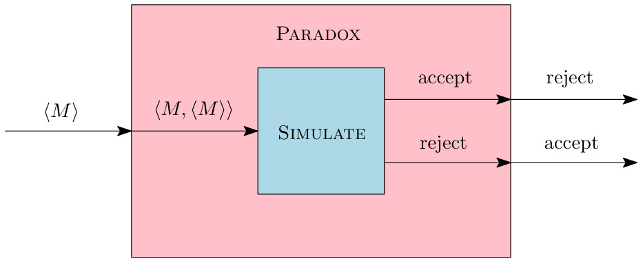
PARADOX built on SIMULATE: the outputs are crossed over, so the machine does the opposite of what it is told.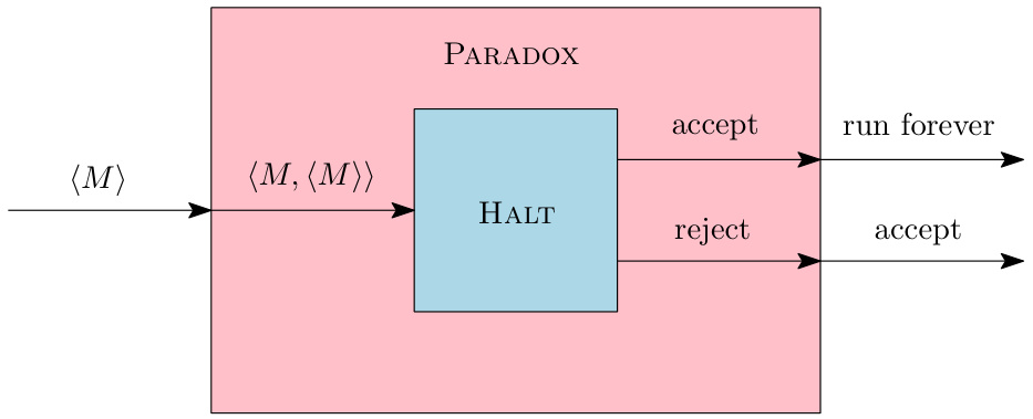
PARADOX built on HALT: accept becomes run-forever, and the same crossing produces the same contradiction.Look at the two diagrams together. The construction is identical; only the box in the middle and one output label change. That is the shape to remember.
Not a hard problem, or one awaiting a cleverer algorithm. No perfect infinite-loop detector, no perfect static analyser for arbitrary runtime behaviour, ever, in any language. Two ingredients made it work, both from the previous unit: programs can be encoded as data, and a machine can be handed its own encoding.
Learning outcomes
- prove-the-halting-problem-unsolvable: Prove that no algorithm decides whether an arbitrary program halts on an arbitrary input.
- apply-cantor-diagonalization: Construct a diagonal language and prove no Turing machine semidecides it.
Concepts
- halting-problem: proves the Halting Problem is algorithmically impossible
- algorithmic-unsolvability: establishes undecidability of program simulation and halting
- turing-semidecidable-language: shows that both simulation and halting are semidecidable but not decidable
Reductions spread unsolvability
Diagonalization is hard work, and you only need it once. After that, reduce.
The definition
Given two languages \(L_{\text{old}}, L_{\text{new}} \subseteq \Sigma^*\), we say \(L_{\text{old}}\) reduces to \(L_{\text{new}}\) — meaning \(L_{\text{new}}\) is at least as hard as \(L_{\text{old}}\) — written
\[L_{\text{old}} \leq_m L_{\text{new}}\]
if there exists a computable function \(f\) such that for all \(x \in \Sigma^*\),
\[x \in L_{\text{old}} \iff f(x) \in L_{\text{new}}\]
The \(m\) in \(\leq_m\) stands for many-to-one. The requirement that \(f\) be computable — a machine that always halts — is what makes the argument carry anything.
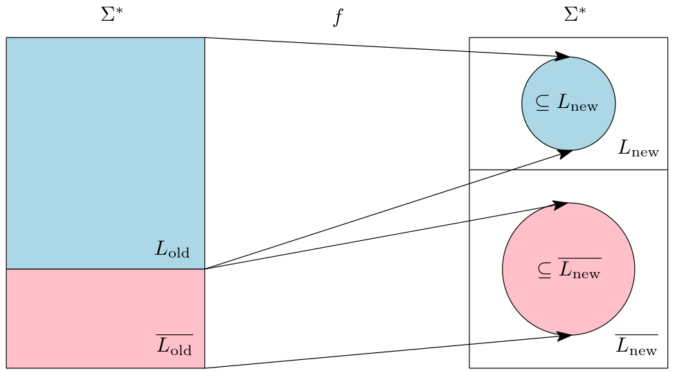
The picture is the intuition: the reduction must turn an instance of \(L_{\text{old}}\) with answer yes into an instance of \(L_{\text{new}}\) with answer yes, and an instance with answer no into one with answer no.
The consequences
If \(L_{\text{old}} \leq_m L_{\text{new}}\), then:
- if \(L_{\text{old}}\) is undecidable, then so is \(L_{\text{new}}\);
- if \(L_{\text{old}}\) is not Turing-semidecidable, then neither is \(L_{\text{new}}\);
- if \(L_{\text{new}}\) is decidable, then so is \(L_{\text{old}}\).
The worked example
Prove HALT impossible again, this time by reduction rather than paradox. Assume HALT is algorithmically possible. Then build:
SIMULATE(<M, w>)
1. result <- HALT(<M, w>)
2. if result = reject then reject        # M runs forever on w
3. elseif result = accept then
4.     Simulate M on w
5.     if M accepts w then accept        # M accepts w
6.     elseif M rejects w then reject    # M rejects w
Line 2 is what makes this terminate: if HALT says \(M\) does not halt, we answer immediately instead of simulating forever. If HALT is an algorithm, then SIMULATE is an algorithm too, terminating in all cases. But we proved SIMULATE is algorithmically impossible. Hence HALT is algorithmically impossible.
We reduce the known-hard problem to the new problem. Building an \(f\) that maps the new problem into the known-hard one proves nothing — it says the new problem is no harder than something impossible, which is empty. This is the most common error in the topic. To check yourself, write out the imagined decider and see which problem it ends up deciding.
Learning outcomes
- build-a-reduction: Use a many-one reduction to transfer unsolvability from a known problem to a new one.
- prove-the-halting-problem-unsolvable: Prove that no algorithm decides whether an arbitrary program halts on an arbitrary input.
Concepts
- many-one-reduction: defines mapping reductions and uses them to reduce simulation to halting
Which questions about machines are solvable?
With reductions available, we can survey the questions people actually want to ask about programs. The source gives two lists, and the interesting thing is what separates them.
Algorithmically solvable
- Given a TM \(M\), does \(M\) have at least 481 states?
- Given a TM \(M\), does \(M\) take more than 481 steps on input \(\epsilon\)?
- Given a TM \(M\), does \(M\) take more than 481 steps on some input?
- Given a TM \(M\), does \(M\) take more than 481 steps on all inputs?
- Given a TM \(M\), does \(M\) ever move its head more than 481 tape cells away from the left endmarker on input \(\epsilon\)?
They all share a feature: a bound. “More than 481 steps on \(\epsilon\)?” — simulate for 482 steps and look. That simulation always halts, because the step count is fixed in advance. “At least 481 states?” is read straight off the description. Bounded questions are decidable, however awkward the bound is to compute.
Algorithmically unsolvable
- Given a TM \(M\) and an input string \(w\), is \(w \in L(M)\)?
- Given a TM \(M\), is \(L(M)\) nonempty?
- Given a TM \(M\), is \(L(M) = \Sigma^*\)?
- Given two TM’s \(M_1\) and \(M_2\), is \(L(M_1) = L(M_2)\)?
- Given two TM’s \(M_1\) and \(M_2\), is \(L(M_1) \subseteq L(M_2)\)?
- Given two TM’s \(M_1\) and \(M_2\), is \(L(M_1) \cap L(M_2)\) nonempty?
- Given a TM \(M\) and an input string \(w\), does \(M\) use a finite amount of tape?
These share a different feature: quantification over all inputs. Is \(L(M)\) nonempty? That asks about every string. Are \(L(M_1)\) and \(L(M_2)\) equal? Again, every string. No finite amount of simulation settles any of them, because a machine that has not accepted yet may still accept later. Each is proved unsolvable by reduction from a problem we already have.
The move to practise
Given a new question about a machine, ask first whether a finite amount of simulation could settle it.
- If yes, it is probably decidable — and you should say how much simulation.
- If no, look for the reduction, and remember which direction it runs.
The pattern behind the whole list: anything a finite check settles is decidable; anything requiring knowledge of behaviour on all inputs generally is not.
Learning outcomes
- classify-tm-properties: Decide whether a question about a Turing machine’s behaviour is solvable or unsolvable.
- build-a-reduction: Use a many-one reduction to transfer unsolvability from a known problem to a new one.
Concepts
- algorithmic-unsolvability: lists decidable bounded-step questions and undecidable behavioural properties
- turing-decidable-language: contrasts solvable bounded properties with undecidable behavioural ones
The limits of computation
Looking back over the unit, you can now define an algorithm formally, place a problem in the right solvability class, and prove unsolvability four ways: counting, diagonalization, self-reference, reduction.
The four techniques form a progression worth holding onto.
- Counting proves unsolvable problems exist without naming one.
- Diagonalization names one.
- Self-reference reaches the problem people actually care about.
- Reduction turns one result into unlimited results, and is what you will actually use.
Stepping back over the module: the previous unit built a model of computation from a person with a pencil, and found it strong enough to do anything a computer can. This unit took the same model and found its edge — and by the Church-Turing thesis, that edge is not a limitation of Turing machines. It is the limit of computation, and no faster hardware or better language moves it.
Learning outcomes
- define-algorithm-formally: Give the formal definition of an algorithm as a Turing machine that halts on every input.
- classify-decidable-semidecidable-computable: Distinguish Turing-decidable, Turing-semidecidable and Turing-computable, and place a problem in the right class.
- state-the-church-turing-thesis: State the Church-Turing thesis and explain why it is a hypothesis rather than a theorem.
- argue-by-cardinality: Use a counting argument to show that most decision problems are not even semidecidable.
- apply-cantor-diagonalization: Construct a diagonal language and prove no Turing machine semidecides it.
- prove-the-halting-problem-unsolvable: Prove that no algorithm decides whether an arbitrary program halts on an arbitrary input.
- build-a-reduction: Use a many-one reduction to transfer unsolvability from a known problem to a new one.
- classify-tm-properties: Decide whether a question about a Turing machine’s behaviour is solvable or unsolvable.
Conclusion
Algorithms are formally equivalent to Turing machines that always halt on all inputs.
The intuitive account — a mechanical procedure of finite steps needing no insight — becomes a machine that decides a language or computes a function. Termination on every input is what the formalization pins down.
Cardinality differences prove that the vast majority of computational problems cannot even be semidecided.
Machines are countable because each is a finite string; decision problems are uncountable because each is a real number in \([0,1]\). Most problems have no program at all.
Diagonalization and self-reference reveal undecidability explicitly.
Flipping the diagonal of the machines-by-strings table names a language no machine semidecides. Handing a machine its own description kills both
SIMULATEandHALT.Reductions propagate unsolvability from one problem to the next.
Once one problem is known hard, a computable mapping in the right direction makes the next one hard for free. This is how the list of undecidable questions about machines grows.
The boundary is a property of computation, not of Turing machines.
By the Church-Turing thesis, no faster hardware and no better language moves it. Real tools cope by approximating, restricting the language, or answering “don’t know” — and knowing which of the three a tool has chosen is the useful form of everything proved here.