Introduction

Lambda Calculus

2026-08-19 09:00

Where we are

What this unit assumes

You have written programs in an imperative language.

Variables, assignment, loops, arrays.

This unit works against that experience.

The experiment

Remove the assignment statement.

What is left?

The answer is: everything. Nothing computable is lost. But making that case takes the whole module, and this unit only sets it up.

What you will be able to do

1. Say what functional programming is.
2. Contrast how the two styles associate names with values.
3. Explain why evaluation order does not change the result.
4. Express repetition as recursion.
5. Pass a function as an argument, return one as a result.
6. Describe how data is built explicitly.
7. Place functional programming in the 1936 computability results.
8. Say why the λ calculus is the core.

Why another way to program

The four differences

• what a name means
• why execution order stops mattering
• how repetition happens without a loop
• how data is built, and why functions are values

Then: where these ideas came from, and what the λ calculus is.

One decision, many consequences

Every difference in this unit follows from a single decision:

what a name is allowed to mean.

What functional programming is

The definition

Functional programming is an approach to programming based on function calls as the primary programming construct.

Why the theory is so clean

It forms a bridge between formal methods in computing and their application.

The reason it has such a clean theory is that it started as theory.

This is not a style someone designed and then found a theory for. It is a theory that turned out to be a style. The history section makes this concrete.

Names and values

Start with a calculator

A calculator does arithmetic on numbers.

Its limitation: no way to generalise a calculation.

To reuse it with different values, re-enter the whole thing.

Names fix that

We write a program using names to stand for values in general.

Then run it with the names taking particular values from the input.

The program does not change. Only the input does.

Both styles agree so far.

The imperative rule

A variable is a changeable association between a name and values.

<command1> ;
<command2> ;
<command3> ;

Each command is typically an assignment:

<name> := <expression>

In imperative languages…

The same name may be associated with different values.

The functional rule

A program is an expression — nested function calls:

<function1>(<function2>(<function3> ... ) ... ))

Names are introduced only as formal parameters, and given values by calls supplying actual parameters.

Once bound, never rebound.

In functional languages…

A name is only ever associated with one value.

What this costs you

To know what a name means imperatively, you must know when you are asking.

Functionally, you look at where it was bound.

Time does not enter.

Execution order stops mattering

The swap

T := X;
X := Y;
Y := T

T depends on X, X depends on Y, Y depends on T.

Any change in the sequence changes what happens.

Same commands, different programs

X := Y;
T := X;
Y := T

sets X to Y

T := X;
Y := T;
X := Y

sets Y to X

Imperative languages have fixed execution orders.

The functional case

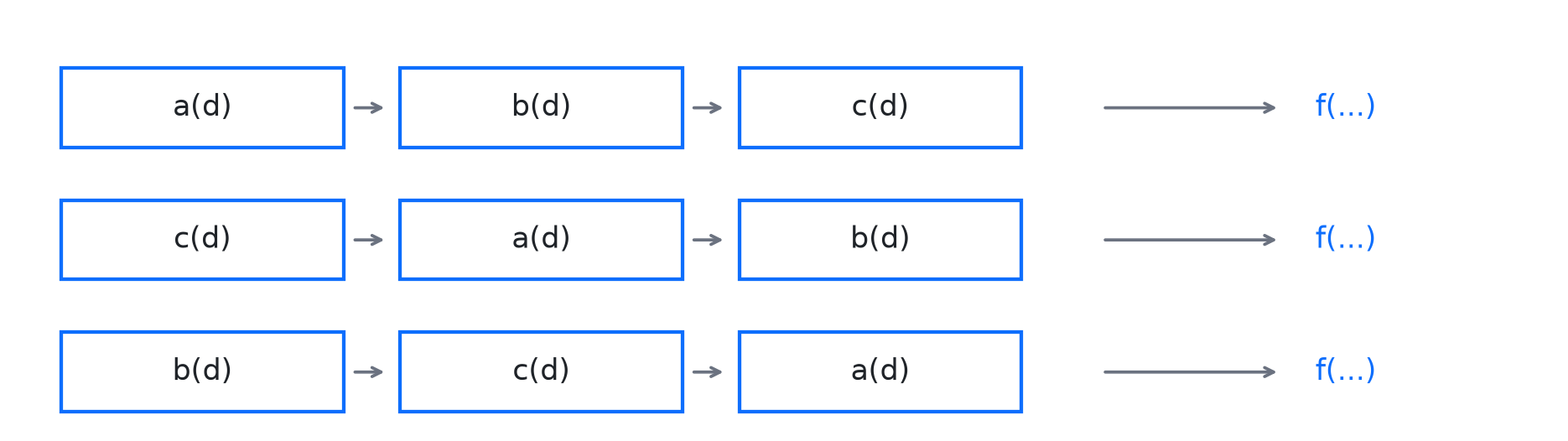
Function calls cannot change values associated with shared names.

\[F(A(D),\ B(D),\ C(D))\]

The order of A(D), B(D), C(D) does not matter — none of them can change D.

In functional languages…

There is no necessary execution order.

Programs still run in some order. It just does not affect the result.

This is what allows reordering and parallel evaluation with no extra machinery — there is no shared state to protect.

One caveat

Order does not affect the result.

It can affect whether evaluation terminates.

Unit 2 makes this precise. Unit 4 depends on it completely.

Repetition without loops

The imperative loop

Summing N elements of A — not this:

SUM1 := A[1];
SUM2 := SUM1 + A[2];

but this:

I := 0;
SUM := 0;
WHILE I < N DO
BEGIN
    I := I + 1;
    SUM := SUM + A[I]
END

The functional version

FUNCTION SUM(A:ARRAY [1..N] OF INTEGER; I,N:INTEGER):INTEGER;
BEGIN
    IF I > N THEN
    SUM := 0
    ELSE
    SUM := A[I] + SUM(A,I+1,N)
END

Each call creates new local versions of A, I and N.

Watch it unfold

B[1] + SUM(B,2,M) =
B[1] + B[2] + SUM(B,3,M)
...
B[1] + B[2] + ... + B[M] + SUM(B, M+1, M)
B[1] + B[2] + ... + B[M] + 0

The correspondence is exact

• the loop’s index → an argument, different each call
• the loop’s accumulator → a returned value
• the loop’s test → the base case, I > N

The variable that “changes” is really a sequence of values. Recursion makes it explicit.

A question deferred

This works because SUM can refer to itself by name.

In the pure λ calculus, a name is an abbreviation, not a reference.

Unit 4 is about getting recursion back.

Data structures, and functions as values

Data is written whole

No assignment means sub-structures cannot be changed one at a time.

Functional languages provide explicit representations for data structures.

No arrays. Nested structures like lists instead, defined recursively.

In LISP the same representation is used for functions and data structures. That coincidence is not an accident, and it comes back in unit 2.

What that buys

• one standard format for displaying structures
• one standard format for storing them
• no globals — every structure is passed in and passed back

Calls get bigger. In exchange, the flow of data is visible.

Functions are values

Functional languages allow functions to be treated as values.

Many imperative languages let you pass a sub-program in.

Few let you pass one back.

Deliberately illegal Pascal

FUNCTION ARITH(OP:OPTYPE):FUNCTION;
FUNCTION SUM(X,Y:INTEGER):INTEGER; BEGIN SUM := X+Y END;
FUNCTION DIFF(X,Y:INTEGER):INTEGER; BEGIN DIFF := X-Y END;
BEGIN
    CASE OP OF
    ADD: ARITH := SUM;
    SUB: ARITH := DIFF;
    END
END

ARITH(ADD)(3, 4)

ARITH(ADD) produces a function; (3, 4) applies it.

Why these are one idea

If functions are values, a structure holding two things can be a function that, given a selector, returns one of them.

Data stops needing its own mechanism.

That is the whole content of unit 3.

Where these ideas came from

The logical background

• Propositional calculus — true/false, and/or/not, names for truth values
• Predicate calculus — non-logical values, predicates, quantifiers
• Peano’s number theory — numbers as 0 and the successor function, proofs by induction

Unit 3 builds the naturals exactly as Peano did.

Inherited, not invented

Within these calculi:

• name–value associations are unchanging
• expressions have no necessary evaluation order

Both properties we met earlier were already there.

1931

Russell and Whitehead try to derive mathematics from logic.

Hilbert asks for a proof that it is consistent and complete.

Gödel: any system powerful enough to describe arithmetic is necessarily incomplete.

1936 — three answers at once

• Turing’s Turing machines
• Kleene’s recursive function theory
• Church’s λ calculus

Each has simple primitives, simple structuring rules, and — crucially — a proof theory.

All three are equivalent

To each other, and to digital computers.

Church’s thesis: all descriptions of computability are equivalent.

Cannot be proved. Never yet contradicted.

A difference of emphasis

Turing machines

symbol manipulation, assignment, time-ordered evaluation

λ calculus, recursive functions

structured function application, evaluation order independent

Two models of the same class — each looking like one of our two programming styles.

Halting, and Church–Rosser

The halting problem is unsolvable — for Turing machines, and equally for λ expressions.

But Church–Rosser: if different evaluation orders terminate, the results are the same.

And one particular order is more likely to terminate than any other.

From theory to languages

• ALGOL 60 — recursion, call-by-name from the λ calculus
• LISP (McCarthy, 1963) — recursive functions on lists; a program is a list
• SECD machine (Landin) — an abstract interpreter; the calculus can be executed
• ISWIM (Landin) — a pure functional language
• Denotational semantics (Strachey, Scott) — every construct gets a function denotation
• Backus, 1977 — FP systems; imperative style as the obstacle

The point of the history

The λ calculus was a model of computation before it was a programming language.

That is why it can be minimal and still be enough.

The λ calculus underneath

Two mechanisms

Abstraction — generalise an expression by introducing names.

Application — evaluate it by giving names particular values.

No numbers. No booleans. No data structures. No control flow. No recursion.

Why that is enough

• Universal — enough for arbitrary programming language constructs
• Evaluation order independent — so it can model different orders
• Provable — well developed proof techniques
• Simple — easy enough to implement and run as a prototype

Universal machine code

Real languages are notation on top of this core.

Every addition — numbers, conditionals, data, recursion — can be explained by translating it back down.

That translation is what units 2 to 4 actually do.

Summary

The six things to carry away

• Every difference between the styles follows from one decision about names.
• Evaluation order cannot change a functional program’s result.
• Repetition is recursion; data is written whole.
• First-class functions are what make the rest possible.
• Functional programming is rooted in 1936 computability theory.
• The λ calculus is a minimal, universal foundation.

Where next

Elements of Lambda Calculus stops motivating and starts defining.

• the grammar for λ expressions
• the reduction rules that evaluate them
• the first functions, built from nothing

Ending with selectors and pairs — the building blocks units 3 and 4 depend on.