Algorithms and the Limits of Computation
Computation and Turing Machines · v2.2.3
2026-09-25 23:14:10
Where we are
Scope and prerequisites
- The previous unit built the machine, the tape, configurations and \(U\)
- Every construction there answered how; this unit asks whether
- Two threads were left hanging, and both are pulled on here
Halting: nothing forces a stop. Universality: \(U\) simulates, does not decide.
Outline of key topics
- The formal definition of algorithm
- Turing-decidable, Turing-computable, Turing-semidecidable
- The Church-Turing thesis
- Four techniques: counting, diagonalization, self-reference, reduction
- Which questions about machines are solvable
From what machines do, to what they cannot
The question the unit answers
Are Turing machines powerful enough to model any conceivable algorithm?
The order of the argument
- define algorithm precisely
- count, and find more problems than machines
- diagonalize, and construct a specific problem no machine solves
- use self-reference to prove the Halting Problem unsolvable
- use reductions to spread unsolvability
Each technique is stronger than the one before.
Scope of the unit
- Everything proved unsolvable here is a question about machines
- Does this machine halt; does it accept anything; do two machines agree
- That keeps the unit self-contained
What exactly is an algorithm?
Definition — algorithm, informally
An algorithm is an effective, systematic, mechanical method for a given problem.
- A finite number of instructions
- Produces the result in a finite number of steps
- Can be carried out by a human with only paper and pen
- Requires no insight, intuition or ingenuity
Clause 2: the termination requirement
Every result in this unit depends on termination in finitely many steps.
- A procedure that may fail to terminate does not satisfy the definition
- Deciding and semideciding differ on this clause alone
Two kinds of problem
Decision problems
Input \(w\), output yes or no.
Yes means \(w \in L\).
Given a chess configuration, can the player to move win?
Function computation
Input \(w\), output \(f(w)\).
Given a social graph, what is the shortest chain between two people?
Two definitions follow: one for languages, one for functions.
What the informal definition leaves open
- Clause 2 rules out non-termination by fiat
- A Turing machine carries no such guarantee
- Reconciling the two is what the formal definitions do
Decidable, semidecidable, computable
Turing-decidable languages
\(M\) decides \(L \subseteq \Sigma^*\) iff for all \(w \in \Sigma^*\):
\[\begin{cases} M \text{ accepts } w, & \text{if } w \in L, \\ M \text{ rejects } w, & \text{if } w \notin L. \end{cases}\]
- A language is Turing-decidable, or recursive, iff some TM decides it
- Every input gets a verdict; no input runs forever
Turing-computable functions
For \(f : \Sigma^* \to \Sigma^*\), a machine computes \(f\) iff for all \(w \in \Sigma^*\):
\[(q_0, \triangleright w) \vdash^{*} (q_{\text{acc}}, \triangleright f(w))\]
- A function is Turing-computable iff some TM computes it
- Again, on every input
Turing-semidecidable languages
\(M\) semidecides \(L\) iff for all \(w \in \Sigma^*\):
\[\begin{cases} M \text{ accepts } w, & \text{if } w \in L, \\ M \text{ rejects } w \text{ or runs forever}, & \text{if } w \notin L. \end{cases}\]
- Turing-semidecidable, or recursively enumerable, iff some TM semidecides it
- A yes answer arrives; a no answer may never arrive
The asymmetry is what separates semideciding from deciding.
Which of these is an algorithm?
| Type of computation | Always halt? |
|---|---|
| TMs for decidable languages | ✓ |
| TMs for computable functions | ✓ |
| TMs for semidecidable languages | ✗ |
- Algorithm — a TM for a decidable language or a computable function
- Algorithmic solvability — Turing-decidability or Turing-computability
- Algorithmic unsolvability — the negation of both
Why semidecidability is excluded
- A procedure that might not stop is not an algorithm
- A great deal of real software is exactly that
- “Semidecidable” does not mean “solvable given patience”
If the machine has not accepted yet, nothing has been learned.
The Church-Turing thesis
The statement
The Church-Turing thesis, in four phrasings:
- Any algorithm can be executed by a Turing machine
- Anything that can be computed can be computed by a Turing machine
- A function is effectively calculable iff it is Turing-computable
- Turing machines can do anything describable as “purely mechanical”
Why it cannot be proved
- One side is formal: Turing machines, defined precisely
- The other is informal: what could be done mechanically
- No proof crosses that gap
- The evidence: every model proposed computes the same functions
Why the thesis is needed here
- Without it, the result is a fact about one formalism
- With it, a fact about computation, and about every language
- Every “no algorithm exists” is “no Turing machine exists”, plus the thesis
Definition — the complement of a language
For \(L \subseteq \Sigma^*\):
\[\overline{L} = \{\, w \in \Sigma^* \mid w \notin L \,\}\]
- the strings over the same alphabet that are not in \(L\)
- A decider for \(L\) answers yes exactly where a decider for \(\overline{L}\) answers no
Property 1 — the complement of a decidable language
If \(L\) is Turing-decidable, then \(\overline{L}\) is Turing-decidable.
DECIDE_NOT_L(w)
1. result <- DECIDE_L(w)
2. if result = accept then
3.     reject
4. else
5. acceptDECIDE_Lhalts on every input, so this does too- Swapping the verdict is the whole construction
One decider serves both, with the answers exchanged.
Property 2 — when the complement is not semidecidable
If \(L\) is semidecidable and undecidable, \(\overline{L}\) is not semidecidable.
DECIDE_L(w)
1. run SEMI_L(w) and SEMI_NOT_L(w)
   in parallel
2. if SEMI_L accepts then
3.     accept
4. elseif SEMI_NOT_L accepts then
5. reject- Suppose \(\overline{L}\) were semidecidable too
- Every \(w\) lies in \(L\) or in \(\overline{L}\), so exactly one side accepts
- That side accepts in finite time, so this halts on every input
It would decide \(L\) — contradicting the assumption that \(L\) is undecidable.
Counting machines against problems
Theorem — more problems than machines
There are strictly more decision problems than there are Turing machines.
The machines can be listed
- A Turing machine is a finite object: states, alphabet, transition table
- Each one can be written out as a finite string
- The machines can therefore be arranged in a single list
Every program in every language appears somewhere on it.
The decision problems cannot
- A decision problem fixes a yes-or-no answer for every string in \(\Sigma^*\)
- More such assignments than entries in any list of machines
The conclusion
Each machine semidecides at most one language, and problems outnumber machines.
- Most decision problems are not Turing-semidecidable
- Not only undecidable, but not even semidecidable
- This argument constructs nothing: it exhibits no specific problem
The solvable problems form a vanishingly small part of the whole.
Diagonalization constructs an undecidable problem
The intuition
Showing a list incomplete requires one object it cannot contain.
- Make it differ from the first entry at the first position
- From the second entry at the second position, and so on
- It cannot then equal entry \(i\) for any \(i\)
Each entry is excluded at the cost of a single disagreement.
Why it is called diagonalization
- A grid: machines down the side, inputs across the top
- Entry \(i\)’s behaviour is row \(i\); position \(i\) within it is column \(i\)
- The chosen disagreements are the cells \((i, i)\) — the diagonal
Step 1 — build the table
| TM | \(w_1\) | \(w_2\) | \(w_3\) | \(w_4\) | \(w_5\) |
|---|---|---|---|---|---|
| \(M_1\) | 1 | 0 | 0 | 1 | 0 |
| \(M_2\) | 0 | 0 | 1 | 0 | 0 |
| \(M_3\) | 0 | 1 | 1 | 1 | 1 |
| \(M_4\) | 1 | 1 | 0 | 1 | 0 |
| \(M_5\) | 0 | 1 | 0 | 0 | 0 |
A 1 where the machine accepts. Every semidecidable language is a row.
Step 2 — read the diagonal and flip it
\[L_d = \{w_i \mid w_i \notin L(M_i)\}\]
\[d_i = \begin{cases} 1 & \text{if } \text{table}_{ii} = 0, \\ 0 & \text{if } \text{table}_{ii} = 1. \end{cases}\]
- The diagonal above is \(1, 0, 1, 1, 0, \ldots\)
- Flipped, it is \(0, 1, 0, 0, 1, \ldots\)
Step 3 — derive the contradiction
Suppose \(L_d = L(M_k)\) for some \(M_k\). Ask whether \(M_k\) accepts \(w_k\).
Case 1 — \(M_k\) accepts \(w_k\)
\[\begin{eqnarray} &\implies& w_k \notin L_d \\ &\implies& w_k \notin L(M_k) \\ &\implies& M_k \text{ does not accept } w_k \end{eqnarray}\]
Case 2 — \(M_k\) does not accept \(w_k\)
\[\begin{eqnarray} &\implies& w_k \in L_d \\ &\implies& w_k \in L(M_k) \\ &\implies& M_k \text{ accepts } w_k \end{eqnarray}\]
Each branch concludes the opposite of its own assumption.
Loops, simulation, and the Halting Problem
Definition — the Halting Problem
\[\text{HALT} = \{\, \langle M, w \rangle \mid M \text{ halts on } w \,\}\]
- \(M\) a machine, \(w\) an input, encoded as one string
- The answer is yes exactly when that machine halts on that input
\(\text{HALT}\) is the problem; HALT is a hypothetical algorithm deciding it.
Looping needs no complexity
Three machines over \(\Sigma = \{a\}\), one state each, none halting.
| \(\triangleright\) | \(a\) | \(\square\) | |
|---|---|---|---|
| \(M_1\): \(q_0\) | \((q_0, \rightarrow)\) | \((q_0, \rightarrow)\) | \((q_0, \rightarrow)\) |
| \(M_2\): \(q_0\) | \((q_0, \rightarrow)\) | \((q_0, a)\) | \((q_0, \square)\) |
| \(M_3\): \(q_0\) | \((q_0, \rightarrow)\) | \((q_0, \leftarrow)\) | \((q_0, \leftarrow)\) |
Undecidability is not caused by complexity.
Definition — the acceptance problem
\[\text{ACCEPT} = \{\, \langle M, w \rangle \mid M \text{ accepts } w \,\}\]
- \(M\) is a Turing machine and \(w\) an input, paired as one string
- The answer is yes exactly when that machine accepts that input
ACCEPT is semidecidable
SIMULATE(<M, w>)
1. Simulate TM M on input string w
2. if M accepts w then
3.     accept
4. elseif M rejects w then
5. reject- If \(M\) accepts, this accepts; if \(M\) rejects, it rejects
- If \(M\) runs forever, it runs forever alongside \(M\)
This procedure exists: it is what a universal machine does.
The question is whether ACCEPT is decidable
SIMULATE(<M, w>)
1. Simulate TM M on input string w
2. if M accepts w then
3.     accept
4. else
5. reject- The change is one word:
elseif M rejects whas becomeelse - The third outcome disappears with it
Where the first version runs forever alongside \(M\), this one rejects.
What the else branch demands
The else branch must establish that \(M\) does not accept \(w\).
- That includes the case where \(M\) never halts at all
- And it must do so without waiting for \(M\)
PARADOX, built on SIMULATE
PARADOX(<M>)
1. result <- SIMULATE(<M, <M>>)
2. if result = accept then
3.     reject
4. elseif result = reject then
5.     accept
Then invoke PARADOX(<PARADOX>) — the machine is handed its own encoding.
The two cases for SIMULATE
Case 1
\[\begin{eqnarray} & & \texttt{PARADOX} \text{ accepts} \\ &\implies& \texttt{SIMULATE} \text{ rejects} \\ &\implies& \texttt{PARADOX} \text{ rejects} \\ &\implies& \text{Contradiction} \end{eqnarray}\]
Case 2
\[\begin{eqnarray} & & \texttt{PARADOX} \text{ rejects} \\ &\implies& \texttt{SIMULATE} \text{ accepts} \\ &\implies& \texttt{PARADOX} \text{ accepts} \\ &\implies& \text{Contradiction} \end{eqnarray}\]
ACCEPT is semidecidable, not decidable. Simulation stays possible.
Deciding halting is impossible
HALT(<M, w>)
1. if M halts on w then
2.     accept
3. else
4. reject- Simulating \(M\) settles lines 1–2: a halt is reached and accepted
- Lines 3–4 are the branch no simulation reaches
Rejecting requires establishing that \(M\) never halts.
PARADOX, built on HALT
PARADOX(<M>)
1. result <- HALT(<M, <M>>)
2. if result = accept then
3.     run forever
4. elseif result = reject then
5.     accept
\[\small \begin{eqnarray} & & \texttt{PARADOX} \text{ accepts} \\ &\implies& \texttt{HALT} \text{ rejects} \\ &\implies& \texttt{PARADOX} \text{ runs forever} \\ &\implies& \text{Contradiction} \end{eqnarray}\]
\[\small \begin{eqnarray} & & \texttt{PARADOX} \text{ runs forever} \\ &\implies& \texttt{HALT} \text{ accepts} \\ &\implies& \texttt{PARADOX} \text{ accepts} \\ &\implies& \text{Contradiction} \end{eqnarray}\]
The two constructions side by side
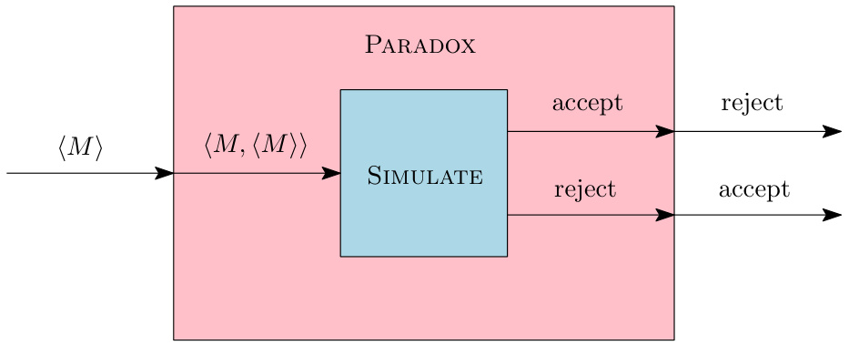
PARADOX on SIMULATE: the outputs are crossed over.
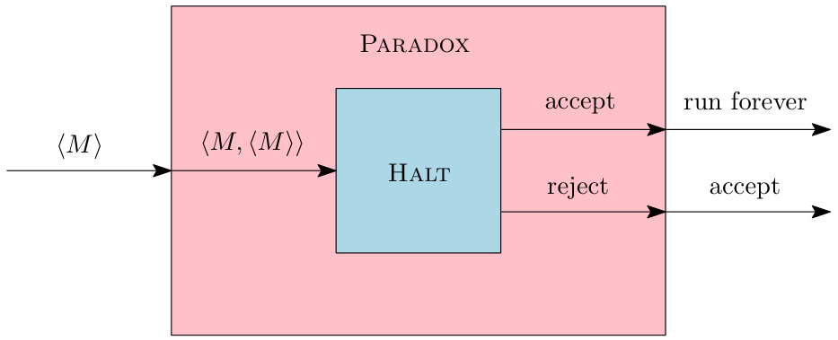
PARADOX on HALT: accept becomes run-forever.
Identical construction; the middle box and one label change.
What this rules out
- Not a hard problem, and not one awaiting a cleverer algorithm
- No perfect loop detector, no perfect static analyser, in any language
- Two ingredients: programs encode as data, and a machine can be handed its own
Reductions spread unsolvability
Definition — many-one reduction
\[L_{\text{old}} \leq_m L_{\text{new}}\]
if there exists a computable function \(f\) such that for all \(x \in \Sigma^*\):
\[x \in L_{\text{old}} \iff f(x) \in L_{\text{new}}\]
\(f\) must be computable, or the argument carries nothing.
What the reduction must do
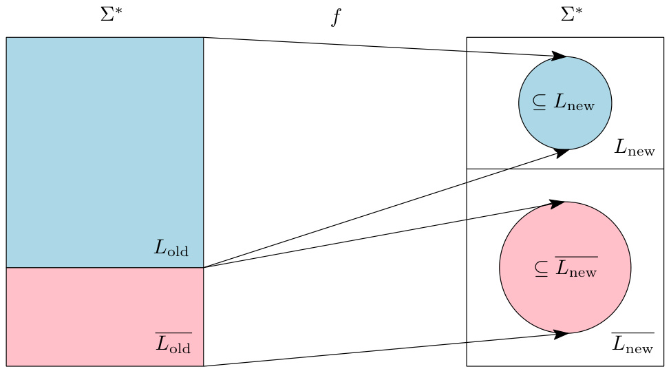
- yes-instances of \(L_{\text{old}}\) map into \(L_{\text{new}}\)
- no-instances map into its complement
- both halves must land correctly
The consequences
If \(L_{\text{old}} \leq_m L_{\text{new}}\):
- if \(L_{\text{old}}\) is undecidable, so is \(L_{\text{new}}\)
- if \(L_{\text{old}}\) is not semidecidable, neither is \(L_{\text{new}}\)
- if \(L_{\text{new}}\) is decidable, so is \(L_{\text{old}}\)
HALT again, by reduction
SIMULATE(<M, w>)
1. result <- HALT(<M, w>)
2. if result = reject then
3.     reject
4. elseif result = accept then
5.     Simulate M on w
6.     if M accepts w then
7.         accept
8.     elseif M rejects w then
9.         reject
Lines 2–3 are what make this terminate.
Direction is everything
- Reduce the known-hard problem to the new problem
- Mapping the new problem into the known-hard one proves nothing
- To check: write the imagined decider, see what it decides
This is the most common error in the topic.
Which questions about machines are solvable?
Algorithmically solvable
- Does \(M\) have at least 481 states?
- Does \(M\) take more than 481 steps on input \(\epsilon\)?
- Does \(M\) take more than 481 steps on some input? On all inputs?
- Does \(M\) move more than 481 cells from the endmarker on \(\epsilon\)?
Each carries a bound: simulate for 482 steps and look.
Algorithmically unsolvable
- Given \(M\) and \(w\), is \(w \in L(M)\)?
- Is \(L(M)\) nonempty? Is \(L(M) = \Sigma^*\)?
- Given \(M_1\) and \(M_2\): is \(L(M_1) = L(M_2)\)? Is \(L(M_1) \subseteq L(M_2)\)?
- Is \(L(M_1) \cap L(M_2)\) nonempty?
- Given \(M\) and \(w\), does \(M\) use a finite amount of tape?
Each quantifies over all inputs; no finite simulation settles it.
How to classify a new question
Ask whether a finite amount of simulation could settle it.
- If yes, it is probably decidable — state how much simulation
- If no, look for the reduction, and check which direction it runs
A finite check settles it: decidable. Behaviour on all inputs: generally not.
Summary
The four techniques
- Counting establishes they exist, without constructing one
- Diagonalization constructs one explicitly
- Self-reference settles the Halting Problem
- Reduction transfers an established result to further problems
Each is stronger than the one before.
The limits of computation
- An algorithm is a TM that halts on every input
- Decidable, semidecidable, and neither — only the first has algorithms
- Most decision problems are not even semidecidable
- ACCEPT and HALT are semidecidable but not decidable
- By the Church-Turing thesis, the edge is not the machine’s
The limit of computation: no hardware or language moves it.